Local Features
Interest point detection
keypoint detection, feature detection
Characteristics of Good Features
-
Repeatable
The same feature can be found in several images despite geometric and photometric transformations
-
Distinct
Captures recognizably different information that allows it to be distinguished
-
Efficient
Quantity: (number of features « number of image pixels); compact
-
Local
A feature occupies a relatively small area of the image (therefore robust to clutter and occlusion).
Goal: Repeatability of Interest Point Detector
Goal: Descriptor Distinctiveness
Descriptors must provide some invariance to geometric and photometric differences between the two views.
Goal: Descriptor Distinctiveness
Look for unusual regions $\rightarrow$ leads to unambiguous matches in other images
At unique regions, shifting the window in any direction causes a big change $\rightarrow$ corner
The Math Behind Corner Detection
$E(u, v) = \sum_{(x,y)\in W}[I(x+u, y+v) - I(x,y)]^2$
We expect $E(u, v)$ to be large.
Consider only samll shift:
$I(x+u, y+v)$
$ = I(x,y) + {\partial I \over \partial x}u + {\partial I \over \partial y}v + higher~order~terms$
$ \approx I(x,y) + {\partial I \over \partial x}u + {\partial I \over \partial y}v$
$ = I(x,y) + I_xu + I_yv $
$E(u, v) = \sum_{(x,y)\in W} [I_xu + I_yv]^2$
$E(u, v) = Au^2 + 2Buv + Cv^2 = \begin{bmatrix} u & v\end{bmatrix}\begin{bmatrix} A & B \\ B & C \end{bmatrix}\begin{bmatrix} u \\ v\end{bmatrix}$
Coefficients in second moment matrix $H = \begin{bmatrix} A & B \\ B & C \end{bmatrix}$ controls the shape of the resulting ellipse.
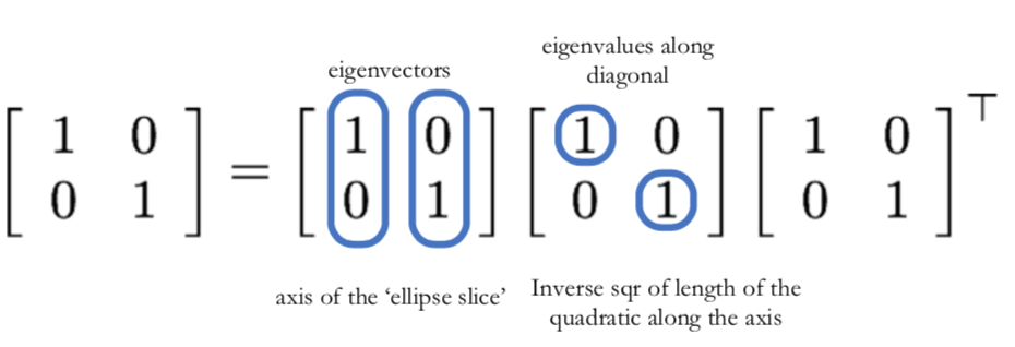
Ellipse axes orientation determined by the eigenvectors of H
Ellipse axes length determined by the eigenvalues of H
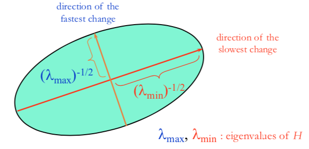
eigenvalue $\lambda_\pm={1\over2}[(h_{11} + h_{22}) \pm \sqrt{4h_{12}h_{21}+(h_{11}-h_{22})^2}]$
eigenvectors $\begin{bmatrix} h_{11}-\lambda & h_{12} \\ h_{21} & h_{22}-\lambda \end{bmatrix}\begin{bmatrix}x \\ y\end{bmatrix}$
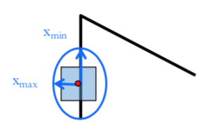
- $x_{max}$ = direction of largest increase in $E$
- $\lambda_{max}$ = amount of increase in direction $x_{max}$
- $x_{min}$ = direction of smallest increase in $E$
- $\lambda_{min}$ = amount of increase in direction $x_{min}$
Converting Eigenvalues to Corners
Use the smallest eigenvalue as the response function $R=min(\lambda_1, \lambda_2)$
Getting eigenvalues (even in our 2x2 scenario is slow because need to take square roots)
A more efficient way is $R = \lambda_1\lambda_2 - \kappa(\lambda_1 + \lambda_2)^2$
$detM = \lambda_1\lambda_2$
$traceM = \lambda_1 + \lambda_2$
$det (\begin{bmatrix}a & b \\ c & d\end{bmatrix}) = ad-bc$
$trace (\begin{bmatrix}a & b \\ c & d\end{bmatrix}) = a+d$
“Cornerness” Functions
Harris & Stephens: $R=det(M) - \kappa trace^2(M)$ $\kappa$ is a small constant, often ~0.04 to 0.06
Kanade & Tomasi: $R=min(\lambda_1, \lambda_2)$
Nobel: $R={det(M) \over trace(M) + \epsilon}$ $\epsilon$ is a small positive constant to prevent dividing by small values close to 0
Weighting the Derivatives
We weight derivatives based on its distance from the center pixel
$H=\sum_{(x, y)\in W} w_{x, y} \begin{bmatrix} I_x^2 & I_xI_y \\ I_xI_y & I_y^2\end{bmatrix}$
Invariance and Equivariance
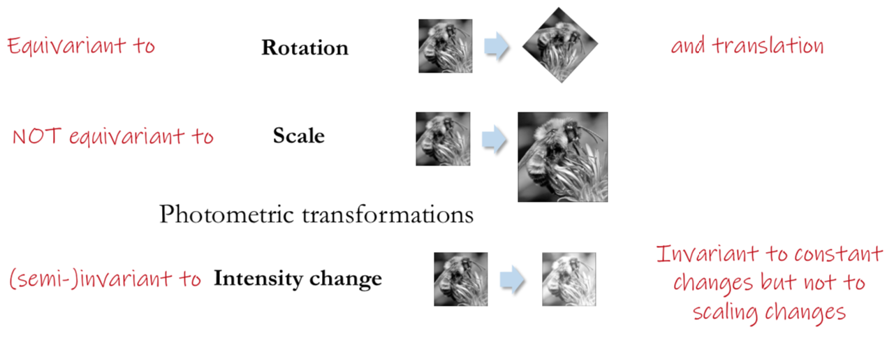
Invariance: image is transformed and corner locations do not change
Equivariance: if we have two transformed versions of the same image, corners should be detected in corresponding locations
Corner locations should be
Equivariant to Geometric transformations
Invariant to Photometric transformations
Invariant to geometric transformations
What happens if image is translated?
-
Derivatives, H obtained through convolution, which is translation equivariant
-
Eigenvalues based only on derivatives so cornerness is invariant
Harris Corner Detector
- Compute gradient at each point in the image
- Compute H matrix for each image window to get their cornerness scores.
- Find points whose surrounding window gave large corner response (f> threshold)
- Take the points of local maxima, i.e., perform non-maximum suppression
Non-maximum Supression
(Simple) Non-Maximum Suppression
Iteratively search for “max” values, then zero-out everything in the surrounding window.
Problem:
- Uneven distribution of interest points in areas of higher contrast
Adaptive Non-Maximum Suppression
Pick features which are both local maxima and whose response is significantly greater (e.g. 10%) than all neighbours within radius r
Invariancy
Thus Harris corner detection location is equivariant to translation, and response is invariant to translation
Corner response depends only eigenvalues so is invariant to rotation
The Harris corner detector (both locations and probability of detection) is invariant to additive changes in intensity, i.e., Changes in overall “Brightness”
It is not invariant to scaling of intensity $I’ \rightarrow \alpha I$, i.e., Changes in “Contrast”
Not invariant to scaling
Conclusion
Harris corners are invariant to geometric transformations such as translation, rotation, semi-invariant to photometric transformations (brightness changes but not contrast) and non-invariant to scaling
What happens to eigenvalues and eigenvectors when a patch rotates?
-
Eigenvectors represent the direction of maximum / minimum change in appearance, so they rotate with the patch
-
Eigenvalues represent the corresponding magnitude of maximum/minimum change so they stay constant
Corner response is only dependent on the eigenvalues so is invariant to rotation
Corner location is as before equivariant to rotation.
Harris Corners – Why so complicated?
It is NOT enough to check for regions with lots of gradients in x and y.
A diagonal line would satisfy that criteria
What are Local Features Good For?
- Matching in Computer Vision
- Estimating Correspondence between Views
- Automatic Mosaicing / Panoramas
- 3D Reconstruction
- Augmented Reality
- Object Recognition
- Stereo Vision
Automatic scale selection
Harris corner detector is not scale invariant, so how can we detect if it’s a corner or an edge.
When looking for corners, find the scale that gives a local maximum of f
Can use fixed window size with a Gaussian pyramid
Laplacian of Gaussian (LoG)
1D
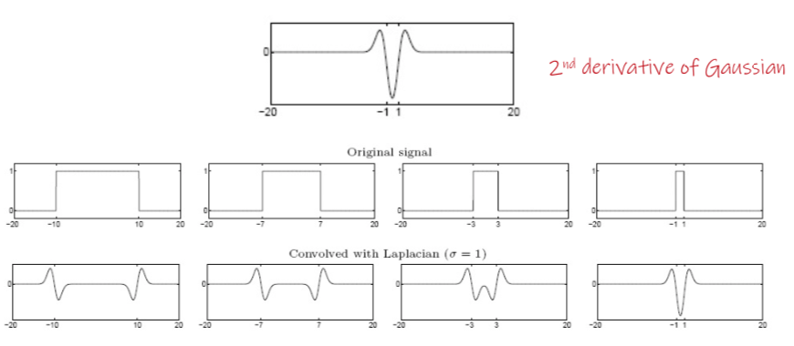
Highest response when the signal has the same characteristic scale as the filter
2D

very similar to a difference of Gaussians – i.e. a Gaussian minus a slightly smaller Gaussian